modelling-with-statcan-workflow • osem

library(osem)
library(dplyr)
library(statcanR)
library(ggplot2)

This is a vignette to describe the process of how to run the model, create forecasts, and create hindcasts using data from Statistics Canada via the implemented statcan dictionary within osem.

Specification

We use a specification for illustrative purposes only. Our specification contains the following four modules/equations:

specification <- dplyr::tibble(
    type = c(
      "d",
      "n"
    ),
    dependent = c(
      "EmiCO2Industry",
      "IndProd"
    ),
    independent = c(
      "HICP_GAS + HICP_Energy + IndProd",
      "GAS"

    )
  )
print(specification)
#> # A tibble: 2 × 3
#>   type  dependent      independent                     
#>   <chr> <chr>          <chr>                           
#> 1 d     EmiCO2Industry HICP_GAS + HICP_Energy + IndProd
#> 2 n     IndProd        GAS

Load statcan dictionary

statcan_dict <- osem::dict_statcan

The statcan dictionary contains a different set of variables than found within eurostat. Due to the way Statistics Canada’s R package pulls data we need to include all the same headers found within the eurostat dictionary in the statcan dictionary to help with data consistency.

print(colnames(statcan_dict))
#>  [1] "model_varname"                                        
#>  [2] "full_name"                                            
#>  [3] "database"                                             
#>  [4] "dataset_id"                                           
#>  [5] "freq"                                                 
#>  [6] "GEO"                                                  
#>  [7] "Seasonal adjustment"                                  
#>  [8] "North American Industry Classification System (NAICS)"
#>  [9] "North American Product Classification System (NAPCS)" 
#> [10] "Prices"                                               
#> [11] "Type of fuel"                                         
#> [12] "Products and product groups"
print(colnames(osem::dict))
#>  [1] "model_varname" "full_name"     "database"      "variable_code"
#>  [5] "dataset_id"    "var_col"       "freq"          "geo"          
#>  [9] "unit"          "s_adj"         "nace_r2"       "ipcc_sector"  
#> [13] "cpa2_1"        "siec"

From the default dictionary, we use the EDGAR variable “EmiCO2Industry” and reset the country in the column geo to CA and then add it to the statcan dictionary:

osem::dict %>% 
  dplyr::filter(model_varname == "EmiCO2Industry") %>% 
  dplyr::mutate(geo = "CA") %>% 
  dplyr::bind_rows(statcan_dict,.) -> statcan_dict_ready

Perform modelling

Now let’s model the equations we have specified and perform some forecasting.

model <- run_model(specification = specification, 
                   dictionary = statcan_dict_ready, 
                   primary_source = "download",
                   quiet = TRUE, 
                   plot = FALSE)

model
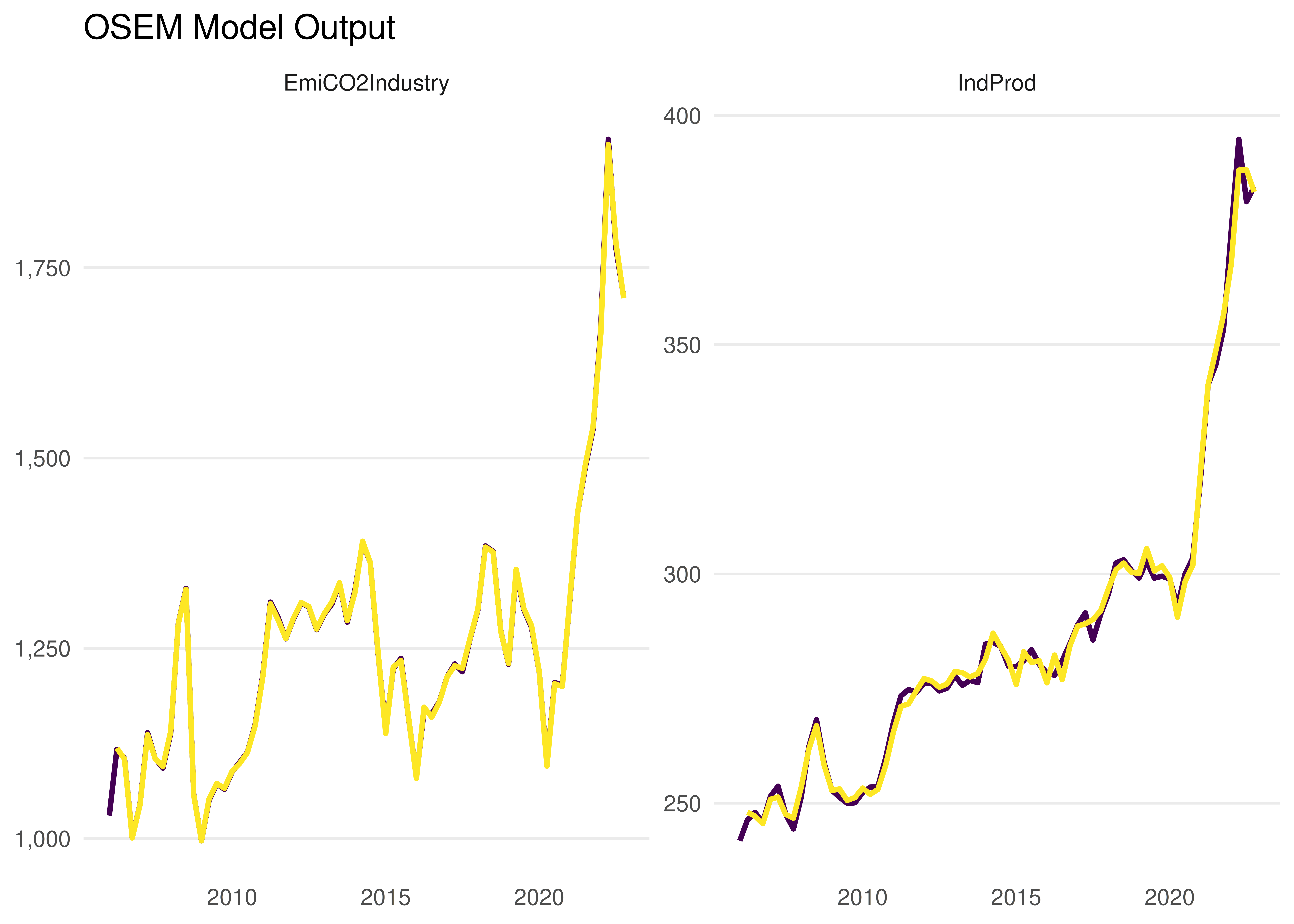
#> OSEM Model Output
#> -----------------------
#> 
#> Estimation Options:
#> Sample: 2006-01-01 to 2022-10-01
#> Max AR Considered: 4
#> Estimation Option: ardl
#> 
#> Relationships considered: 
#> # A tibble: 2 × 3
#>   Model `Dep. Var.`    `Ind. Var`                      
#> 1     1 EmiCO2Industry HICP_GAS + HICP_Energy + IndProd
#> 2     2 IndProd        GAS                             
#> 
#> 
#> Relationships estimated in the order:  2,1
#> 
#> Diagnostics:
#>  # A tibble: 1 × 8
#>   `Dependent Variable` AR    ARCH     `Super Exogeneity`   IIS   SIS     n
#>   <chr>                <chr> <chr>    <chr>              <int> <int> <int>
#> 1 IndProd              0.448 0.001*** 0.013**                1     4    67
#> # ℹ 1 more variable: `Share of Indicators` <dbl>

Forecasting

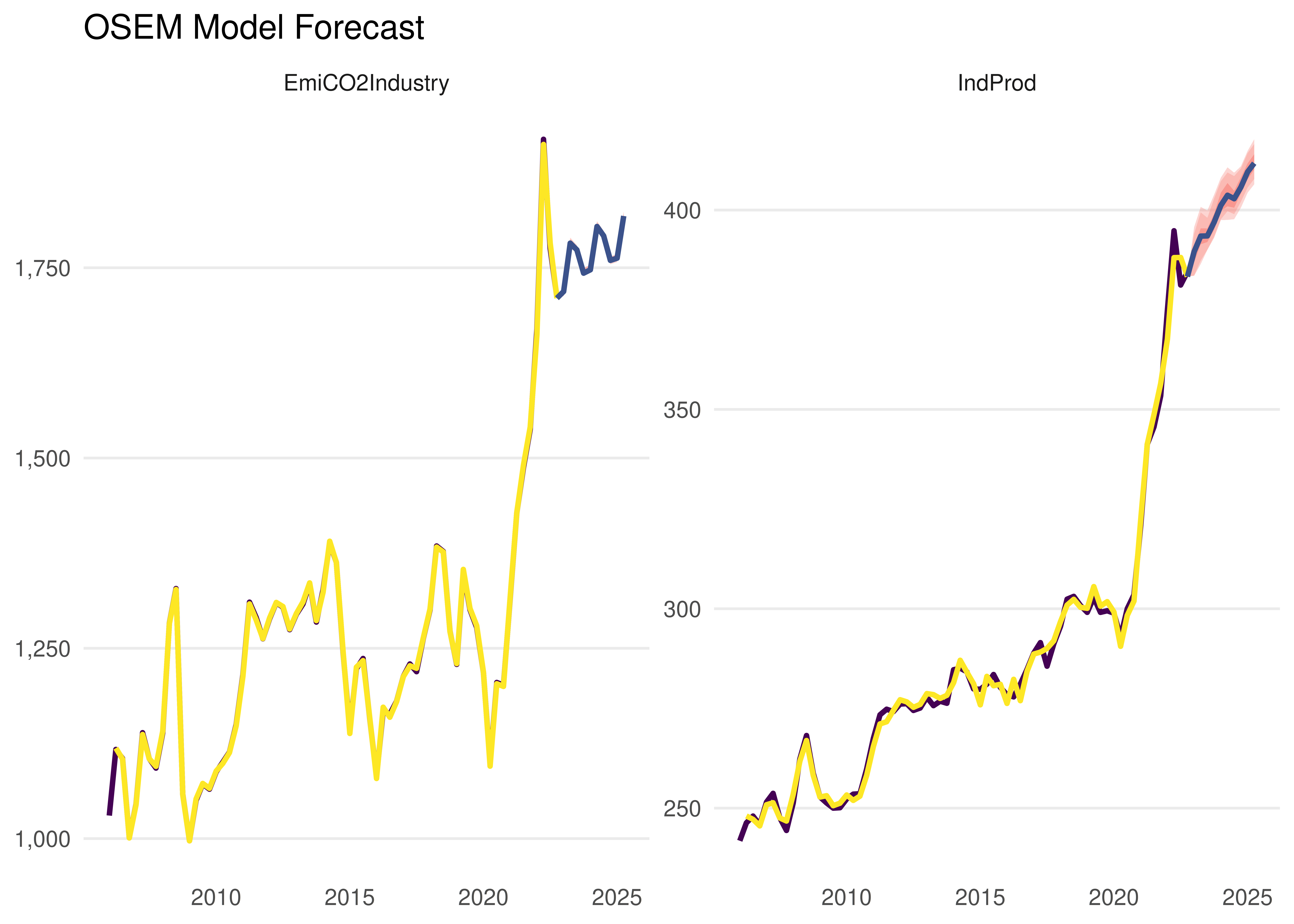
forecast <- forecast_model(model = model, plot = FALSE)
#> No exogenous values provided. Model will forecast the exogenous values with an AR4 process (incl. Q dummies, IIS and SIS w 't.pval = 0.001').
#> Alternative is exog_fill_method = 'last'.

plot(forecast)